好,好数学,要看不懂了
https://zaixiang.notion.site/Diffusion-Models-for-Deep-Generative-Learning-24ccc2e2a11e40699723b277a7ebdd64
\(K L(p, q)=\log \frac{\sigma_2}{\sigma_1}+\frac{\sigma^2+\left(\mu_1-\mu_2\right)^2}{2 \sigma_2^2}-\frac{1}{2}\)
high-quality samples using diffusion models
connections among diffusion models and:
high-quality image synthesis using diffusion probabilistic models
Best results: obtained by training on a weighted variational bound designed according to a novel connection between diffusion probabilistic models and denoising score matching with Langevin dynamics
Transformers are expressive(contain no inductive bias that prioritizes local interactions compared to CNNs)
However, long sequences are computationally infeasible in Transformers (e.g hi-res images can result in an embedding with so high dimensions which makes the computations cost high)
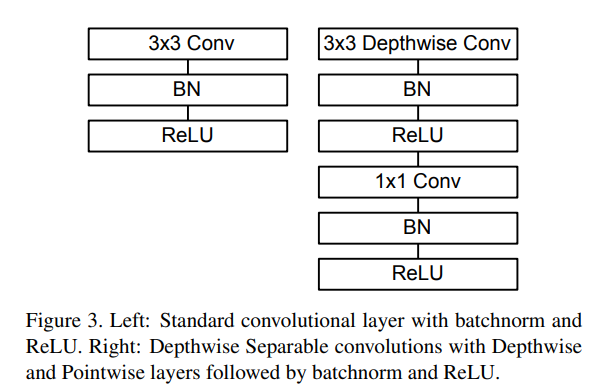
2 Stage Method: CNNs can learn a context-rich vocab of image constituents (and lower the dimension)
Transformers in turn efficiently model their composition
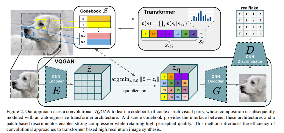
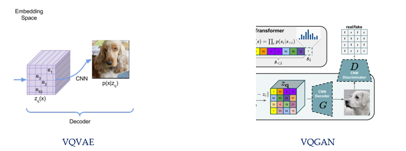
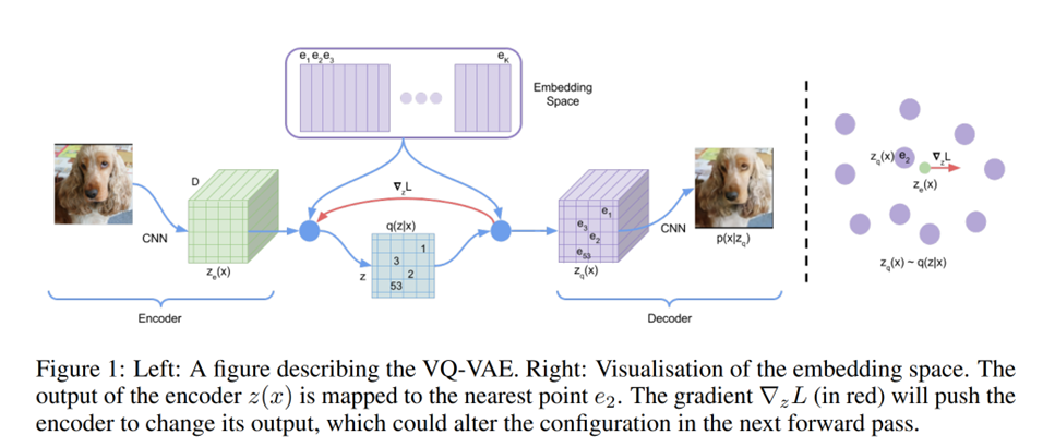
Model architecture of VQVAE
Model architecture of VQGAN
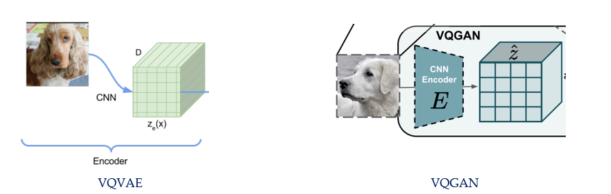
Same Encoder(CNN)
Turning an image to Tensors
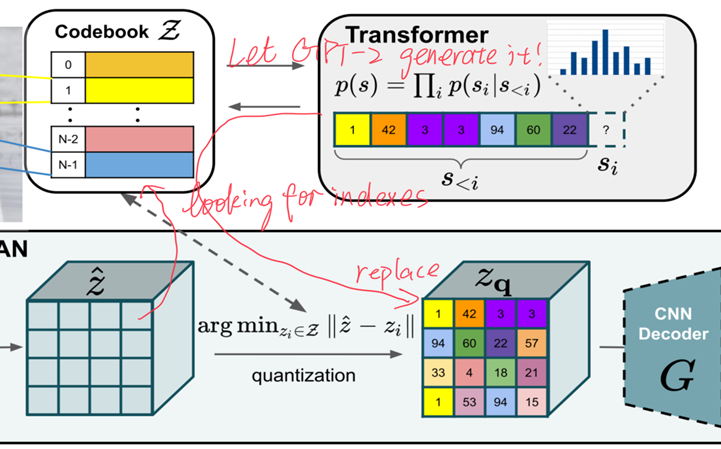
VQVAE finds the nearest embedding e_k in [Embedding Space] and codebook updates with the encoder(loss)
VQGAN uses a 2-stage approach
Stage 1: use VAE to learn the Codebook Z
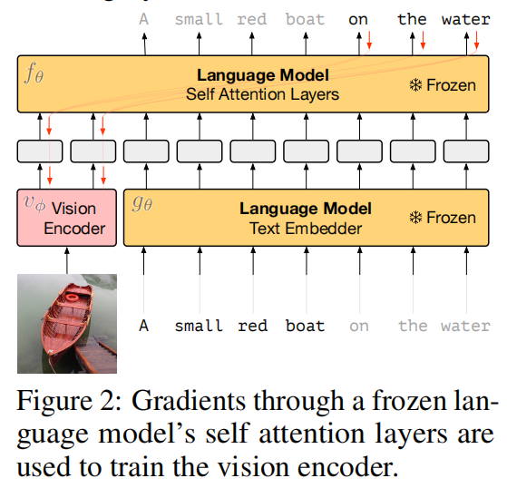
Stage 2: use Transformer(GPT-2) to generate latent code
VQVAE sends z_q (x) into CNN decoder to generate output
VQGAN sends z_q (x) into CNN decoder to generate output, too. But with a CNN discriminator (GAN)
Patch-based (high-res images are too large)
Sending signals to codebook, encoder and decoder
Loss function in VQ is:
\[\begin{aligned} \mathcal{L}_{\mathrm{VQ}}(E, G, \mathcal{Z})=\|x-\hat{x}\|^{2} +\left\|\operatorname{sg}[E(x)]-z_{\mathrm{q}}\right\|_{2}^{2} +\left\|\operatorname{sg}\left[z_{\mathrm{q}}\right]-E(x)\right\|_{2}^{2} . \end{aligned}\]Here, \(\|x-\hat{x}\|^{2}\) corresponds to Reconstruction Loss (GAN), the \(\left\|\mathrm{sg}[E(x)]-z_{\mathrm{q}}\right\|_{2}^{2}\) trains the codebook, and \(\left\|\mathrm{sg}\left[z_{\mathrm{q}}\right]-E(x)\right\|_{2}^{2}\) trains the encoder. P.S. the \(s g[x]\) means stopgradient, which means we don’t calculate the gradient of the input \(x\).
Loss function in Discriminator \(D\) (GAN) is: \(\mathcal{L}_{\mathrm{GAN}}(\{E, G, \mathcal{Z}\}, D)=[\log D(x)+\log (1-D(\hat{x}))]\)
Then the whole model can be described as:
\[\begin{aligned} \mathcal{Q}^{*}=\underset{E, G, \mathcal{Z}}{\arg \min } \max _{D} \mathbb{E}_{x \sim p(x)} & {\left[\mathcal{L}_{\mathrm{VQ}}(E, G, \mathcal{Z})\right.} \left.+\lambda \mathcal{L}_{\mathrm{GAN}}(\{E, G, \mathcal{Z}\}, D)\right] \end{aligned}\]We combine the loss of generator and discriminator
\[\begin{aligned} \mathcal{Q}^{*}=\underset{E, G, \mathcal{Z}}{\arg \min } \max _{D} \mathbb{E}_{x \sim p(x)} & {\left[\mathcal{L}_{\mathrm{VQ}}(E, G, \mathcal{Z})\right.} \left.+\lambda \mathcal{L}_{\mathrm{GAN}}(\{E, G, \mathcal{Z}\}, D)\right] \end{aligned}\]And here, lambda is used to balance the 2 losses:
\[\lambda=\frac{\nabla_{G_{L}}\left[\mathcal{L}_{\mathrm{rec}}\right]}{\nabla_{G_{L}}\left[\mathcal{L}_{\mathrm{GAN}}\right]+\delta}\]And \(\delta=10-6\) prevents this lambda from \(0 / 0\). (numerical stability)
\(\nabla \mathrm{GL}[\cdot]\) denotes the gradient of its input w.r.t. the last layer \(\mathrm{L}\) of the decoder.
In Stage 1 we successfully learn a good codebook(it can generate a good image which passes the discriminator!)
Then we use the codebook to replace E(x) i.e. 𝑧 ̂. Take a look back at the Figure 2 (GPT-2 autoregressively generate the next code in 𝑧_𝑞).
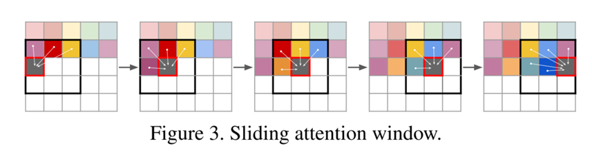
What about the large images? (remember we want to generate hi-res images!)
If the z_q has too much slots to fill, in Transformer it will be a huge array which takes up a lot of resources!
So we need to do some blocking things – a sliding attention window:
In every sliding window, we generate the next code autoregressively using the information within it (resource-friendly).
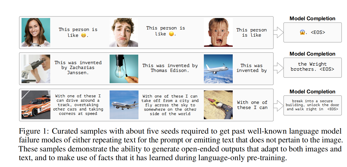
Another thing is conditioned synthesis: We can give the model some information (which is called Condition) to guide it in generating images.
The Condition can be from a single label to even another image.
How it operates:
Train Batch EM | Train Batch F1 | Validation/Train EM | Validation/Train F1 |
---|---|---|---|
Train Batch EM | Train Batch F1 | Train EM | Train F1 |
---|---|---|---|
Train Loss | Validation EM | Validation F1 |
---|---|---|
Train Batch EM | Train Batch F1 | Validation/Train EM | Validation/Train F1 |
---|---|---|---|
Train Batch EM | Train Batch F1 | Validation/Train EM | Validation/Train F1 |
---|---|---|---|
捞干货!
如 figure 1 所示,VQA model 无法处理 “发出声音” 的这部分问题,因为没有输入声音数据看不出来。如果是单声道的话,AQA model 也无法处理“which clarinet” 在发声这种问题,因为没有输入视觉数据。
在这项工作中,我们专注于视听问答(AVQA)任务,旨在回答有关视觉对象、声音及其关联的问题。 为此,本质上需要一个计算模型来具备对丰富的动态视听场景的有效多模态理解和推理能力。 为了促进上述研究,我们构建了一个大规模的时空音乐 AVQA (MUSIC-AVQA) 数据集。
考虑到音乐表演是典型的多模态场景,由丰富的视听成分及其交互组成,适合用于探索 audio-visual scene understanding and reasoning。
因此,我们从 YouTube 收集了大量用户上传的音乐表演视频:
为了解决上述 AVQA 任务,我们分别从空间和时间基础的角度考虑这个问题。
这篇 paper 所做工作:
在这项工作中,我们调查视听问题是一个转向问题,旨在通过充分利用多感官内容来回答有关视频的问题。 为了促进这项任务,我们构建了一个大规模的 MUSIC-AVQA 数据集,该数据集由 45,867 个问答对组成,跨越视听模式和不同的问题类型。 我们还提出了一个时空接地模型来探索细粒度的场景理解和推理。 我们的结果表明,所有不同的模式都有助于解决 AVQA 任务,并且我们的模型执行最近的 QA 方法,特别是在配备我们提出的模块时。 我们相信我们的数据集可以成为评估细粒度视听场景理解和时空推理的有用测试平台,并有可能激发更多人探索该领域。
尽管我们已经取得了相当大的进步,但 AVQA 任务仍有很大的探索空间。 首先,当前数据集的场景更局限于音乐场景,而视听交互更多地存在于日常场景中。 我们将在后续研究中探索更一般场景中的视听推理任务。 我们的模型只是将复杂的场景分解为具体的视听关联。 然而,一些与问题无关的视觉对象或声源涉及到编码的单峰嵌入,可能会引入学习噪声并使解决 QA 任务具有挑战性
如图 4 中所示的失败示例(F)。 为了缓解这个问题,我们可以将每个视频解析为单独的对象和孤立的声音,然后自适应地利用与问题相关的音频和视觉元素来更准确地回答问题。
此外,为了促进时间推理,我们建议突出显示接近问题的关键时间戳。 然而,这样的模块缺乏音频和视觉模态之间的明确时间建模。 更先进的模型可以连接跨模式的时间关联,预计将进一步提高性能。 虽然场景有些局限,但我们认为这是视听推理的第一步,我们相信本文将是该领域的一个良好开端。
发布的 MUSIC-AVQA 数据集是经过策划的,它可能具有仪器和地理区域之间的潜在相关性。 这个问题值得进一步研究和考虑。
我们认为声音及其视源的位置通常反映了视听模态之间的空间关联,因此引入了执行基于注意力的声源定位的空间接地模块,将复杂的场景分解为具体的视听关联。
具体来说,对于每个视频片段 \(V_t\),视觉特征映射 \( f_{v,m}^t \) 和相应的音频特征 \(f^t_a\) ∈ \(R^C\) 构成匹配对。 然后我们随机采样另一个视觉片段,得到它的视觉特征图,它与音频特征 \(f^t_a\) 组成不匹配对。 对于每一对,我们可以计算与声音相关的视觉特征\( f^t_{v,s}\),如下:
其中 σ 是 softmax, (·)⊺ 表示转置算子。 为了防止可能的视觉信息丢失,我们平均池化视觉特征图 ftv,m,得到全局视觉特征 ftv,g。 将两个视觉特征融合为视觉表示:
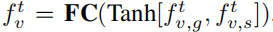
其中 FC 表示全连接层。 然后,结合视觉和音频表示来预测视听对是否匹配:
\(y^{match}\) 表示视听特征是否来自匹配对。即当 \(f_t^v\) 和 \(f_t^a\) 为匹配对时,\(y^{match}\) = 1,否则\(y^{match}\) = 0。\(L_{ce}\) 为交叉熵损失。
需要注意的是,非匹配对只在空间接地模块中使用,即\(f_t^v\) 和 \(f_t^a\)在其他模块中始终是匹配对。
为了突出与问题密切相关的关键时间戳,我们提出了一个时间基础模块,该模块旨在关注不断变化的视听场景中的关键时间段,并捕获和问题相关的音频和视觉嵌入。
具体来说,给定一个\(f_q\)和视听特征
时间基础模块将学习聚合问题感知的音频和视觉特征。 接地音频特征 f¯a 和视觉特征 f¯v 可以计算为:
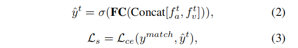
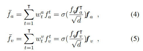
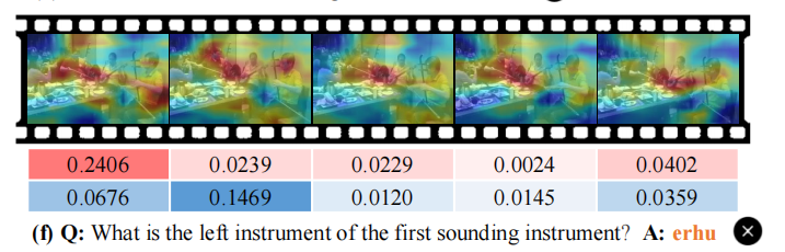
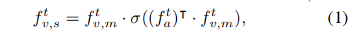
d 是与特征维度大小相同的缩放因子。 显然,该模型将为与所提出的问题更相关的音频和视频片段分配较大的权重。 因此,基于问题的音频/视觉上下文嵌入更能预测正确答案。
Contents credit to Talk from Jacob Menick @ DeepMind.
当以足够的规模进行训练时,自回归语言模型在仅提示几个示例后就表现出学习新语言任务的显着能力。
auto-regressive language models
Auto-regressive transformers 很厉害 balabalabala
它们属于 few-shot learners: 给几个示例就可以学习一样新任务,也不用接着训练(梯度更新)
这样呢,用 prompt 就可以非常快地 adapt to new tasks:
之前的模型基本上不处理文本之外的模式,这里提出 Frozen:
proposed a new model architecture called MobileNets based on depthwise separable convolutions.
investigated some of the important design decisions leading to an efficient model.
demonstrated how to build smaller and faster MobileNets using width multiplier and resolution multiplier by trading off a reasonable amount of accuracy to reduce size and latency.
compared different MobileNets to popular models demonstrating superior size, speed and accuracy characteristics
concluded by demonstrating MobileNet’s effectiveness when applied to a wide variety of tasks.
传统卷积的计算量:(D_FD_FD_KD_KM*N)。其中DF为特征图尺寸,DK为卷积核尺寸,M为输入通道数,N为输出通道数。
计算量 (D_FD_FD_KD_KM)
计算量 (D_FD_FM*N)
总计
比较:
如果看源码的话可以发现这个 ReLU 层用的是 ReLU6:
# from https://github.com/tensorflow/models/blob/master/research/slim/nets/mobilenet/mobilenet_v2.py
activation_fn: Activation function to use, defaults to tf.nn.relu6 if not
specified.
把一个流形用 random matrix T 映射到 n 维空间后用 ReLU 处理,再用 T 的逆矩阵映射回来在低维度造成了信息丢失。高维度看起来其实是还可以的。
最后的那个 ReLU 被换成线性激活函数 -> Linear BottleNeck
类似 ResNet 复用特征:
另外你也可以看到尾部的 RELU6 被换成了 Linear。
与 ResNet 相比,MobileNet V2 由 ResNet 的 0.25 降维变成了 6 倍升维,这样实际上 MobileNet 在网络中间的部分维度是比较大的。 具象起来就比较像纺锤结构。而 Resnet 中间的维度比较小。这样想象一下就可以理解 MobileNet 为什么用 Inverted residuals 这个名字了。
V2 的 block:
网络结构:
NAS(hardware-aware network architecture search)
Squeeze-And-Excite
Small 和 Large 的版本参数
使用 Stride 进行降采样,不使用 pooling。
the linear bottleneck and inverted residual structure(V1)
depthwise separable convolutions (V2)
lightweight attention modules based on squeeze and excitation into the bottleneck structure
hard sigmoid:
Sigmoid:
class hswish(nn.Module):
def forward(self, x):
out = x * F.relu6(x + 3, inplace=True) / 6
return out
class hsigmoid(nn.Module):
def forward(self, x):
out = F.relu6(x + 3, inplace=True) / 6
return out
Source Code: https://github.com/BC-Li/deep_learning_playground
First appeared in Gradient-based learning applied to document recognition
channel 在深度学习的算法学习中,都会提到 channels 这个概念。在一般的深度学习框架的 conv2d 中,如 tensorflow 、mxnet ,channels 都是必填的一个参数。
channels 该如何理解?
一般的RGB图片,channels 数量是 3 (红、绿、蓝);而monochrome图片,channels 数量是 1
一般 channels 的含义是,每个卷积层中卷积核的数量。 为什么这么说呢,看下面的例子:
如下图,假设现有一个为 6×6×3的图片样本,使用 3×3×3 的卷积核(filter)进行卷积操作。此时输入图片的 channels 为 3 ,而卷积核中的 in_channels 与 需要进行卷积操作的数据的 channels 一致(这里就是图片样本,为3)。
网络结构:
net = nn.Sequential(
nn.Conv2d(1,6,kernel_size=5,padding=2),nn.Sigmoid(),
nn.AvgPool2d(kernel_size=2,stride=2),#28*28->14*14
nn.Conv2d(6,16,kernel_size=5,),nn.Sigmoid(),#14*14->10*10
nn.AvgPool2d(kernel_size=2,stride=2),#10*10->5*5
nn.Flatten(),
nn.Linear(16 * 5 * 5,120),nn.Sigmoid(),
nn.Linear(120,84),nn.Sigmoid(),
nn.Linear(84,10)
)
在 GPU 上训练结果:
(colanora_conda_env) [colanora@colanora learning]$ python -u "/home/colanora/learning/lenet.py"
training on cuda:0
/home/colanora/learning/lenet.py:28: DeprecationWarning: `set_matplotlib_formats` is deprecated since IPython 7.23, directly use `matplotlib_inline.backend_inline.set_matplotlib_formats()`
display.set_matplotlib_formats('svg')
<Figure size 350x250 with 1 Axes>
...
loss 0.482, train acc 0.817, test acc 0.791
48381.2 examples/sec on cuda:0
Left: LeNet, Right: AlexNet
alexnet = nn.Sequential(
nn.Conv2d(1, 96, kernel_size=11, stride=4, padding=1),
nn.ReLU(),
nn.MaxPool2d(kernel_size=3, stride=2),
nn.Conv2d(96, 256, kernel_size=5, padding=2),
nn.ReLU(),
nn.MaxPool2d(kernel_size=3, stride=2),
nn.Conv2d(256, 384, kernel_size=3, padding=1),
nn.ReLU(),
nn.Conv2d(384, 384, kernel_size=3, padding=1),
nn.ReLU(),
nn.Conv2d(384, 256, kernel_size=3, padding=1),
nn.ReLU(),
nn.MaxPool2d(kernel_size=3, stride=2),
nn.Flatten(),
nn.Linear(6400, 4096),
nn.ReLU(),
nn.Dropout(),
nn.Linear(4096, 4096),
nn.ReLU(),
nn.Dropout(p=0.5),
nn.Linear(4096, 10),
)
GPU 上训练结果:
(colanora_conda_env) [colanora@colanora learning]$ python -u "/home/colanora/learning/lenet.py"
training on cuda:0
/home/colanora/learning/lenet.py:28: DeprecationWarning: `set_matplotlib_formats` is deprecated since IPython 7.23, directly use `matplotlib_inline.backend_inline.set_matplotlib_formats()`
display.set_matplotlib_formats("svg")
<Figure size 350x250 with 1 Axes>
...
loss 0.323, train acc 0.881, test acc 0.884
1503.4 examples/sec on cuda:0
def nin_block(in_channels, out_channels, kernel_size, strides, padding):
return nn.Sequential(
nn.Conv2d(in_channels, out_channels, kernel_size, strides, padding),
nn.ReLU(),
nn.Conv2d(out_channels, out_channels, kernel_size=1),
nn.ReLU(),
nn.Conv2d(out_channels, out_channels, kernel_size=1),
nn.ReLU(),
)
nin_net = nn.Sequential(
nin_block(1, 96, kernel_size=11, strides=4, padding=0),
nn.MaxPool2d(3, stride=2),
nin_block(96, 256, kernel_size=5, strides=1, padding=2),
nn.MaxPool2d(3, stride=2),
nin_block(256, 384, kernel_size=3, strides=1, padding=1),
nn.MaxPool2d(3, stride=2),
nn.Dropout(0.5),
nin_block(384, 10, kernel_size=3, strides=1, padding=1),
nn.AdaptiveAvgPool2d((1, 1)),
nn.Flatten(),
)
(colanora_conda_env) [colanora@colanora learning]$ python -u "/home/colanora/learning/lenet.py"
training on cuda:0
/home/colanora/learning/lenet.py:28: DeprecationWarning: `set_matplotlib_formats` is deprecated since IPython 7.23, directly use `matplotlib_inline.backend_inline.set_matplotlib_formats()`
display.set_matplotlib_formats("svg")
<Figure size 350x250 with 1 Axes>
...
loss 0.491, train acc 0.819, test acc 0.804
1374.1 examples/sec on cuda:0
# inception-net
class inception_block(nn.Module):
def __init__(self, in_channels, c1, c2, c3, c4, **kwargs):
super(inception_block, self).__init__(**kwargs)
self.p1_1 = nn.Conv2d(in_channels, c1, kernel_size=1)
self.p2_1 = nn.Conv2d(in_channels, c2[0], kernel_size=1)
self.p2_2 = nn.Conv2d(c2[0], c2[1], kernel_size=3, padding=1)
self.p3_1 = nn.Conv2d(in_channels, c3[0], kernel_size=1)
self.p3_2 = nn.Conv2d(c3[0], c3[1], kernel_size=5, padding=2)
# 线路4,3x3最大汇聚层后接1x1卷积层
self.p4_1 = nn.MaxPool2d(kernel_size=3, stride=1, padding=1)
self.p4_2 = nn.Conv2d(in_channels, c4, kernel_size=1)
def forward(self, x):
p1 = torch.nn.functional.relu(self.p1_1(x))
p2 = torch.nn.functional.relu(self.p2_2(torch.nn.functional.relu(self.p2_1(x))))
p3 = torch.nn.functional.relu(self.p3_2(torch.nn.functional.relu(self.p3_1(x))))
p4 = torch.nn.functional.relu(self.p4_2(self.p4_1(x)))
# 在通道维度上连结输出
return torch.cat((p1, p2, p3, p4), dim=1)
b1 = nn.Sequential(
nn.Conv2d(1, 64, kernel_size=7, stride=2, padding=3), nn.ReLU(), nn.MaxPool2d(kernel_size=3, stride=2, padding=1)
)
b2 = nn.Sequential(
nn.Conv2d(64, 64, kernel_size=1),
nn.ReLU(),
nn.Conv2d(64, 192, kernel_size=3, padding=1),
nn.ReLU(),
nn.MaxPool2d(kernel_size=3, stride=2, padding=1),
)
b3 = nn.Sequential(
inception_block(192, 64, (96, 128), (16, 32), 32),
inception_block(256, 128, (128, 192), (32, 96), 64),
nn.MaxPool2d(kernel_size=3, stride=2, padding=1),
)
b4 = nn.Sequential(
inception_block(480, 192, (96, 208), (16, 48), 64),
inception_block(512, 160, (112, 224), (24, 64), 64),
inception_block(512, 128, (128, 256), (24, 64), 64),
inception_block(512, 112, (144, 288), (32, 64), 64),
inception_block(528, 256, (160, 320), (32, 128), 128),
nn.MaxPool2d(kernel_size=3, stride=2, padding=1),
)
b5 = nn.Sequential(
inception_block(832, 256, (160, 320), (32, 128), 128),
inception_block(832, 384, (192, 384), (48, 128), 128),
nn.AdaptiveAvgPool2d((1, 1)),
nn.Flatten(),
)
inception_net = nn.Sequential(b1, b2, b3, b4, b5, nn.Linear(1024, 10))
(colanora_conda_env) [colanora@colanora learning]$ python -u "/home/colanora/learning/lenet.py"
training on cuda:0
/home/colanora/learning/lenet.py:28: DeprecationWarning: `set_matplotlib_formats` is deprecated since IPython 7.23, directly use `matplotlib_inline.backend_inline.set_matplotlib_formats()`
display.set_matplotlib_formats("svg")
loss 0.240, train acc 0.908, test acc 0.896
1669.3 examples/sec on cuda:0
主要是在卷积块后面接了一个跨层的数据通路,把 x 直接跨过去了。
让我们聚焦于神经网络局部:如图 图7.6.2所示,假设我们的原始输入为xx,而希望学出的理想映射为f(x)f(x)(作为 图7.6.2上方激活函数的输入)。 图7.6.2左图虚线框中的部分需要直接拟合出该映射f(x)f(x),而右图虚线框中的部分则需要拟合出残差映射f(x)−xf(x)−x。 残差映射在现实中往往更容易优化。 以本节开头提到的恒等映射作为我们希望学出的理想映射f(x)f(x),我们只需将 图7.6.2中右图虚线框内上方的加权运算(如仿射)的权重和偏置参数设成0,那么f(x)f(x)即为恒等映射。 实际中,当理想映射f(x)f(x)极接近于恒等映射时,残差映射也易于捕捉恒等映射的细微波动。 图7.6.2右图是ResNet的基础架构–残差块(residual block)。 在残差块中,输入可通过跨层数据线路更快地向前传播。
参数:
batch_size = 256
resize = 96
lr, num_epochs = 0.1, 10
(colanora_conda_env) [colanora@colanora learning]$ python -u "/home/colanora/learning/lenet.py"
training on cuda:0
/home/colanora/learning/lenet.py:28: DeprecationWarning: `set_matplotlib_formats` is deprecated since IPython 7.23, directly use `matplotlib_inline.backend_inline.set_matplotlib_formats()`
display.set_matplotlib_formats("svg")
loss 0.012, train acc 0.997, test acc 0.906
2215.3 examples/sec on cuda:0
感觉好像参数环境啥的忘写了,等我有空补一下
开学人就是这么卑微
ResNet将整个拟合函数分为(或者说展开)为两部分:一个简单的线性项和一个复杂的非线性项。
(f(\mathbf{x}) = \mathbf{x} + g(\mathbf{x}).
DenseNet 更进一步,用连接 将函数分解成一个展开式:
(\mathbf{x} \to \left[ \mathbf{x}, f_1(\mathbf{x}), f_2([\mathbf{x}, f_1(\mathbf{x})]), f_3([\mathbf{x}, f_1(\mathbf{x}), f_2([\mathbf{x}, f_1(\mathbf{x})])]), \ldots\right].)
这些展开式用多层展开机连接,实现起来就是用全连接连起来就行了。
稠密网络主要由2部分构成:稠密块(dense block)和过渡层(transition layer)。 前者定义如何连接输入和输出,而后者则控制通道数量,使其不会太复杂。
# DenseNet
def conv_block(input_channels, num_channels):
return nn.Sequential(
nn.BatchNorm2d(input_channels), nn.ReLU(), nn.Conv2d(input_channels, num_channels, kernel_size=3, padding=1)
)
class DenseBlock(nn.Module):
def __init__(self, num_convs, input_channels, num_channels):
super(DenseBlock, self).__init__()
layer = []
for i in range(num_convs):
layer.append(conv_block(num_channels * i + input_channels, num_channels))
self.net = nn.Sequential(*layer)
def forward(self, X):
for blk in self.net:
Y = blk(X)
# 连接通道维度上每个块的输入和输出
X = torch.cat((X, Y), dim=1)
return X
blk = DenseBlock(2, 3, 10)
X = torch.randn(4, 3, 8, 8)
Y = blk(X)
print(Y.shape)
# 由于每个稠密块都会带来通道数的增加,使用过多则会过于复杂化模型。 而过渡层可以用来控制模型复杂度。 它通过 1×1 卷积层来减小通道数,并使用步幅为2的平均汇聚层减半高和宽,从而进一步降低模型复杂度。
def transition_block(input_channels, num_channels):
return nn.Sequential(
nn.BatchNorm2d(input_channels),
nn.ReLU(),
nn.Conv2d(input_channels, num_channels, kernel_size=1),
nn.AvgPool2d(kernel_size=2, stride=2),
)
blk = transition_block(23, 10)
print(blk(Y).shape)
# the same as resnet
# b1 = nn.Sequential(
# nn.Conv2d(1, 64, kernel_size=7, stride=2, padding=3),
# nn.BatchNorm2d(64),
# nn.ReLU(),
# nn.MaxPool2d(kernel_size=3, stride=2, padding=1),
# )
num_channels, growth_rate = 64, 32
num_convs_in_dense_blocks = [4, 4, 4, 4]
blks = []
for i, num_convs in enumerate(num_convs_in_dense_blocks):
blks.append(DenseBlock(num_convs, num_channels, growth_rate))
num_channels += num_convs * growth_rate
if i != len(num_convs_in_dense_blocks) - 1:
blks.append(transition_block(num_channels, num_channels // 2))
num_channels = num_channels // 2
densenet = nn.Sequential(
b1,
*blks,
nn.BatchNorm2d(num_channels),
nn.ReLU(),
nn.AdaptiveMaxPool2d((1, 1)),
nn.Flatten(),
nn.Linear(num_channels, 10),
)
参数:
batch_size = 256
resize = 96
lr, num_epochs = 0.1, 10
(colanora_conda_env) [colanora@colanora learning]$ python -u "/home/colanora/learning/lenet.py"
training on cuda:0
/home/colanora/learning/lenet.py:28: DeprecationWarning: `set_matplotlib_formats` is deprecated since IPython 7.23, directly use `matplotlib_inline.backend_inline.set_matplotlib_formats()`
display.set_matplotlib_formats("svg")
loss 0.147, train acc 0.947, test acc 0.910
2561.6 examples/sec on cuda:0
]]>1.Backbone:翻译为骨干网络的意思,既然说是主干网络,就代表其是网络的一部分,那么是哪部分呢?这个主干网络大多时候指的是提取特征的网络,其作用就是提取图片中的信息,共后面的网络使用。这些网络经常使用的是resnet VGG等,而不是我们自己设计的网络,因为这些网络已经证明了在分类等问题上的特征提取能力是很强的。在用这些网络作为backbone的时候,都是直接加载官方已经训练好的模型参数,后面接着我们自己的网络。让网络的这两个部分同时进行训练,因为加载的backbone模型已经具有提取特征的能力了,在我们的训练过程中,会对他进行微调,使得其更适合于我们自己的任务。
2.Neck:是放在backbone和head之间的,是为了更好的利用backbone提取的特征。
3.Bottleneck:瓶颈的意思,通常指的是网网络输入的数据维度和输出的维度不同,输出的维度比输入的小了许多,就像脖子一样,变细了。经常设置的参数 bottle_num=256,指的是网络输出的数据的维度是256 ,可是输入进来的可能是1024维度的。
4.Head:head是获取网络输出内容的网络,利用之前提取的特征,head利用这些特征,做出预测。
现代神经序列生成模型的构建要么从头开始逐步生成令牌,要么(迭代地)修改以固定长度为界的令牌序列。
在这项工作中,我们开发了 Levenshtein Transformer,这是一种新的部分自回归模型,旨在实现更灵活和更适合的序列生成:
与以前的方法不同,我们模型的原子操作是插入和删除。 它们的组合不仅有助于生成,还有助于序列细化,允许动态长度变化。 我们还提出了一套专门针对它们的新训练技术,由于它们的互补性,有效地利用了一个作为另一个的学习信号。 应用所提出模型的实验在生成(例如机器翻译、文本摘要)和细化任务(例如自动后期编辑)。 我们通过展示由机器翻译训练的 Levenshtein Transformer 进一步证实了我们模型的灵活性,可以直接用于自动后期编辑。
Automatic Post-Editing: (ref).
Automatic Post-Editing (APE) aims to correct systematic errors in a machine translated text.
See also: https://www.statmt.org/wmt17/ape-task.html
在本文中,我们提出了 Levenshtein Transformer (LevT),旨在解决当前解码模型缺乏灵活性的问题。
值得注意的是,在现有框架中,随着解码的进行,生成序列的长度要么是固定的,要么是单调增加的。 这仍然与人类可以修改、替换、撤销或删除其生成文本的任何部分的人类智能不兼容。 因此,LevT 通过打破迄今为止标准化的解码机制并用两个原子操作(插入和删除)替换它来弥补这一差距。
我们使用模仿学习训练 LevT。 结果模型包含两个策略,它们以交替方式执行。 根据经验,我们表明 LevT 在机器翻译和摘要方面取得了与标准 Transformer 模型相当或更好的结果,同时保持了与 (Lee et al., 2018) 类似的并行解码带来的效率优势。 使用这个模型,我们认为解码变得更加灵活。 例如,当解码器被赋予一个空标记时,它会退回到正常的序列生成模型。
另一方面,当初始状态是低质量的生成序列时,解码器充当细化模型。 事实上,我们表明从机器翻译训练出来的 LevT 直接适用于翻译后编辑,无需任何更改。 这对于文献中的任何框架都是不可能的,因为由于模型的归纳偏差,生成和细化被视为两个不同的任务。
LevT 框架中的一个关键组件是学习算法。 我们利用插入和删除的特征——它们是互补的,但也是对抗的。 我们提出的算法称为“双策略学习”。 这个想法是,在训练一个策略(插入或删除)时,我们使用其对手在前一次迭代中的输出作为输入。 另一方面,专家策略被绘制以提供修正信号。 尽管如此,理论上,该学习算法适用于存在双重对抗策略的其他模仿学习场景,在这项工作中,我们主要关注该算法在训练提出的 LevT 模型时的概念验证。
TLDR Version:
我们提出了 Levenshtein Transformer,一种基于插入和删除的神经序列生成模型。
结果模型实现了性能和解码效率,并在一个模型中同时包含了序列生成和refinement。
插入和删除操作可以说更类似于人类编写或编辑文本的方式。
对于未来的工作,有可能将此模型扩展到 human-in-the-loop generation。
HITL refers to systems that allow humans to give direct feedback to a model for predictions below a certain level of confidence.
缺乏大型并行语料库
已有建议:
三角测量
半监督学习
它们仍然需要强大的跨语言信号。
这项工作中我们完全消除了对并行数据的需求,提出了一种完全无监督训练 NMT 的新方法,只依赖于单语语料库。
As for monolingual corpora, parallel and comparable corpora: https://zhuanlan.zhihu.com/p/59514775
Arch:模型建立在最近关于无监督嵌入映射的工作之上,并由一个稍微修改的注意力编码器-解码器模型组成,
Training:该模型可以单独使用去噪和反向翻译的组合在单语语料库上进行训练。
Performance:尽管该方法很简单,但我们的系统在 WMT 2014 法语 → 英语和德语 → 英语翻译中获得了 15.56 和 10.21 BLEU 点。 该模型还可以从小样本量的平行语料库中获益,结合100,000个平行句子分别获得21.81和15.24分。
Open Source:https://github.com/artetxem/undreamt
神经机器翻译 (NMT) 最近已成为机器翻译的主要范式。与传统的统计机器翻译 (SMT) 不同,NMT 系统是端到端训练的,利用连续表示大大缓解稀疏问题,并利用更大的上下文,从而减轻局部性问题。 正因为如此,NMT 在自动指标和人工评估方面都比 SMT 有显着改进。
第二段复读了一遍 abstract 里面的话:
缺乏大型并行语料库
已有建议:
三角测量
半监督学习
它们仍然需要强大的跨语言信号。
补课:端到端(end to end)是个啥东西?:https://www.zhihu.com/question/51435499 see also https://blog.csdn.net/Dontla/article/details/104550858/
在这项工作中:
我们消除了对跨语言信息的需求,并提出了一种新方法
完全无监督的方式训练 NMT 系统,仅依赖单语语料库。
我们的方法基于最近关于无监督跨语言嵌入的工作(Artetxe 等人,2017;Zhang 等人,2017)。
这个方法使用了一个共享 encoder,两个 translation 方向都用了一个不变的跨语料嵌入,这样呢,就可以使用单语数据训练整个系统以重建其输入。 为了学习有用的结构信息,在这个输入中引入了random token swap形式的噪声。 除了去噪,我们还将back translation纳入训练过程以进一步改善结果。
In this work, we propose a novel method to train an NMT system in a completely unsupervised manner. We build upon existing work on unsupervised cross-lingual embeddings (Artetxe et al., 2017; Zhang et al., 2017), and incorporate them in a modified attentional encoder-decoder model. By using a shared encoder with these fixed cross-lingual embeddings, we are able to train the system from monolingual corpora alone, combining denoising and backtranslation. The experiments show the effectiveness of our proposal, obtaining significant improvements in the BLEU score over a baseline system that performs word-by-word substitution in the standard WMT 2014 French-English and German-English benchmarks. Our manual analysis confirms the quality of the proposed system, showing that it is able to model complex cross-lingual relations and produce high-quality translations. Moreover, we show that combining our method with a small parallel corpus can bring further improvements, showing its potential interest beyond the strictly unsupervised scenario.
the whole system can be optimized to:
encoder 学习用独立于语言的方式来组合两种语言的embedding。 decoder 学习到的是把这种表示来解码成他们对应的语言。
推理时把 decoder 换了就行。 encoder 是 language-independent 的,就不用换了。
然而,这种理想的行为受到了这样一个事实的严重影响,即由此产生的训练过程本质上是一个微不足道的复制任务。 因此,该任务的最佳解决方案不需要捕获所涉及语言的任何真正知识,因为会有许多退化的解决方案盲目地复制输入序列中的所有元素。 如果是这种情况,当用于在推理时从一种语言翻译成另一种语言时,系统最多只能进行非常字面的逐字替换。
为了避免退化,就在句子里面加随机噪声。更具体地说,对于 N 个元素的序列,我们进行 N/2 个随机交换。 这样,系统需要了解所涉及语言的内部结构才能恢复正确的词序。 同时,通过阻止系统过度依赖输入序列的词序,我们可以更好地解释跨语言的实际词序差异。
a> denoising:有点像 denoising auto-encoder。就是把某种语言的句子加一些噪声(随机交换一些词的顺序等),然后用 shared encoder 编码加噪声后的句子,最后用该语言的句子解码恢复它。通过最大化重构出的概率来训练 shared encoder 和该语言的 decoder。加噪声的目的是想让 encoder 学会分析语言的结构、提取语义特征,decoder 学一个好的语言模型,而不是仅仅学会复制粘贴;
From: (Notes on Unsupervised Neural Machine Translation:https://zhuanlan.zhihu.com/p/30649985)
背景:尽管有去噪策略,上面的训练过程仍然是一个复制任务,有一些综合改变,最重要的是,每次都涉及一种语言,而不考虑我们在两种语言之间翻译的最终目标。 为了在真正的翻译环境中训练我们的系统,而不违反只使用单语语料库的限制,我们建议采用 Sennrich 等人提出的反向翻译方法。
给定一种语言的输入句子,我们使用具有贪心解码的推理模式系统将其翻译成另一种语言(即应用共享的编码器和另一种语言的解码器)。 这样,我们获得了一个伪平行句子对,并训练系统从这个合成翻译中预测原始句子。
b> back-translation:语言 L1 的句子 s1 先用编码器编码,然后用 L2 decoder 贪心解码出 s2,这样就造出了伪平行句对 (s2, s1),这时只做推断不更新模型参数;然后再用 shared encoder 编码 s2,用 L1 decoder 解码出 s1,这里通过最大化 P(s1|s2) 来训练模型(也就是 shared encoder 和 L1 decoder 的参数)。
(注:back-translation 是 Sennrich 15 年提出来的数据增广的技巧,详见论文 [1511.06709] Improving Neural Machine Translation Models with Monolingual Data 。具体做法是把单语语料用训好的机器学习模型翻译一遍做成伪平行语料,然后把这样的句对也当做训练数据来训模型,其实就是半监督学习的做法。叫 back-translation 是因为假如你增广语料的时候是把 s1 翻译成了 s2,那么训练的时候要用 s2 翻译出 s1 这个方向来训模型。其动机是,目标语言必须始终是真句子才能让翻译模型翻译的结果更流畅、更准确,而源语言即便有少量用词不当、语序不对、语法错误,只要不影响理解就无所谓。其实人做翻译的时候也是一样的:翻译质量取决于一个人译出语言的水平,而不是源语言的水平(源语言的水平只要足够看懂句子即可))
From (Notes on Unsupervised Neural Machine Translation:https://zhuanlan.zhihu.com/p/30649985)
Notes on Unsupervised Neural Machine Translation:https://zhuanlan.zhihu.com/p/30649985
]]>微调大型预训练模型是 NLP 中一种有效的传输机制。 但是如果下游任务太多,就不可能给每一个任务都 fine-tune 再存参数(效率太低了!)这篇论文给出了另外的方案:加一个 adapter 模块。换下游任务的时候只需要调 adapter 里面的参数就可以了,而不是把整个模型里面的参数全给调了。
Adapter modules yield a compact and extensible model; they add only a few trainable parameters per task, and new tasks can be added without revisiting previous ones. The parameters of the original network remain fixed, yielding a high degree of parameter sharing.
we transfer the recently proposed BERT Transformer model to 26 diverse text classification tasks, including the GLUE benchmark.
作者用 BERT 做了 26 个下游任务,跑了 GLUE BENCHMARK.
Adapters attain near state-of-the-art performance, whilst adding only a few parameters per task. On GLUE, we attain within 0.4% of the performance of full fine-tuning, adding only 3.6% parameters per task. By contrast, fine-tuning trains 100% of the parameters per task.
Adapters 基本上靠近 SOTA 了,同时只加了一丢丢参数。GLUE 跑分在 full fine-tuning 的0.4%以内,但只加了 3.6%参数。 full fine-tuning 肯定是每次都要把参数全 train 掉的。
补课:啥是 fine-tuning?https://www.zhihu.com/question/40850491
从预训练模型的迁移在许多 NLP 任务上产生了强大的性能
BERT 是一种在具有无监督损失的大型文本语料库上训练的 Transformer 网络,在文本分类和抽取式问答方面取得了SOTA性能
在本文中,我们讨论了在线设置,其中任务以流的形式到达。
目标是建立一个在所有这些方面都表现良好的系统,但无需为每项新任务训练一个全新的模型。
任务之间的高度共享对于云服务等应用程序特别有用,在这些应用程序中,需要训练模型来解决客户按顺序到达的许多任务。 为此,我们提出了一种迁移学习策略,可以产生紧凑且可扩展的下游模型。
紧凑模型的意思就是多任务处理的时候换任务只需要换一点参数就可以解决新的task。
可扩展模型是那种可以逐步训练来解决新任务的模型,不会忘记以前的任务。
我们的方法在不牺牲性能的情况下产出这样的模型。
NLP 中最常见的两种迁移学习技术是基于特征的迁移和微调。 相反,我们提出了一种基于adapter模块的替代传输方法。 基于特征的迁移涉及预训练实值嵌入向量。 这些嵌入可能位于单词、句子或段落级别。 然后将嵌入馈送到自定义下游模型。 微调包括从预先训练的网络复制权重并在下游任务上调整它们。 最近的工作表明,微调通常比基于特征的迁移更好。
基于特征的迁移和微调都需要为每个任务设置一组新的权重。 如果网络的较低层在任务之间共享,则微调的参数效率更高。 然而,我们提出的适配器调整方法的参数效率更高。 图 1 展示了这种权衡。 x 轴显示每个任务训练的参数数量; 这对应于解决每个额外任务所需的模型大小的边际增加。
从这个图上可以看到效果:基于适配器的调优比 fine-tuning 训练少两个数量级的参数,同时性能差不多。
Adapters 是加在 pre-trained network 层间的模块。
We present a strategy for tuning a large text model on several downstream tasks.
Our strategy has three key properties:
it attains good performance
it permits training on tasks sequentially, that is, it does not require simultaneous access to all datasets
it adds only a small number of additional parameters per task.
These properties are especially useful in the context of cloud services, where many models need to be trained on a series of downstream tasks, so a high degree of sharing is desirable.
为了实现这个特性,我们提出了一个 bottleneck adapter module. 用 adapter 做 tuning 需要向模型里放一点新参数,这些新参数在下游任务里面训练。
在对深度网络进行 vanilla 微调时,会对网络的顶层进行修改。
这是必需的,因为上游和下游任务的标签空间和损失不同。
adapter module 执行更通用的架构修改,以将预先训练的网络重新用于下游任务。 具体来说呢,adapter module 调整涉及将新层注入原始网络。 原始网络的权重保持不变,而新的adapter module层的权重是随机初始化的。正常 fine-tuning中,新的顶层和原始权重是共同训练的。 而在adapter module调整中,原始网络的参数被冻结,因此可能被许多任务共享。
Adapter Module 的两个特点:参数少和 near-identity initialization。
Adapter Module 需要做得很小,这样总模型大小随着 task 增多不会增加太快。
near-identity initialization 是为了模型魔改后还能稳定训练,同时训练开始的时候原网络不受影响。训练的时候 adapter 才会被激活,进而影响整个网络的激活分布。如果你用不到 adapter 也可以直接 ignore 它们。(感觉有点像 plug-in)
在第 3.6 节中,我们观察到一些特定的adapter对网络的影响比其他adapter更大。 我们还观察到,如果初始化偏离恒等函数太远,模型可能无法训练。
我们在 text Transformers 上操作一下 adapter-based tuning. Transformers 在很多领域都是 SOTA 级别。
这篇论文在 2017 年的 standard Transformer 上做了实例化(我 blog 中那个)。
adapter 的架构很多,这篇论文弄了一个比较简单的设计,还试了下更复杂的设计,但最后实验发现效果都差不多。
上图就是我们的 adapter 架构,和加了 adapter 的 transformer 架构。
Transformer 的每一层都包含两个主要的子层:注意力层和前馈层。 两个层后面紧跟着一个投影,将特征大小映射回层输入的大小。
跳过连接(skip-connection)应用于每个子层。
每个子层的输出被送入Layer Norm。
我们在每个子层之后插入两个串行adapter。
适配器总是直接应用于子层的输出,在投影回输入大小之后,但在添加回跳跃连接之前。 然后将适配器的输出直接传递到下一层规范化。
看下 Figure 2 的右边部分。为了限制参数的数量,我们提出了一个瓶颈架构。 adapter 首先将原始 d 维特征投影到较小的维度 m,应用非线性(nonlinearity),然后再投影回 d 维度。 每层添加的参数总数(包括偏差)为 2md + d + m(这玩意咋算的?)。 通过设置 m«d,我们限制了每个任务添加的参数数量; 在实践中,我们使用了大约 0.5 - 8% 的原始模型参数。 瓶颈维度 m 提供了一种简单的方法来权衡性能与参数效率。 adapter 模块本身在内部具有跳过连接。 使用跳跃连接,如果投影层的参数被初始化为接近零,则模块被初始化为近似恒等函数。
除了适配器模块中的层,我们还为每个任务训练新的层规范化参数。 这种技术类似于条件批量标准化 (De Vries et al., 2017)、FiLM (Perez et al., 2018) 和自调制 (Chen et al., 2019),也产生了参数有效适应 一个网络; 每层只有 2d 个参数。 然而,单独训练层归一化参数不足以获得良好的性能,请参见第 3.4 节。
下面展示 Adapter 做到了在文本任务上 parameter efficient transfer.
NLP|谈谈预训练模型中的Adapter结构:https://codewithzichao.github.io/2020/07/02/NLP-%E8%B0%88%E8%B0%88BERT%E4%B8%AD%E7%9A%84Adapter%E7%BB%93%E6%9E%84/
NLP的“第四范式”之Prompt Learning总结:44篇论文逐一梳理:https://blog.csdn.net/c9Yv2cf9I06K2A9E/article/details/120944308
Parameter-Efficient Transfer Learning for NLP *2:https://zhuanlan.zhihu.com/p/261298193
论文笔记 - NLP 预训练模型综述: https://zhuanlan.zhihu.com/p/139015428
论文阅读 | Pre-trained Models for Natural Language Processing: A Survey:https://www.cnblogs.com/shona/p/12546820.html
]]>