This is my reading report for Multimedia Analysis 2021 Spring in USTC.
Design
Overall architecture of the Deconvolution Network is shown below:
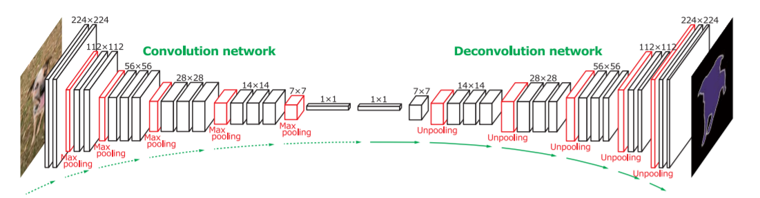
We can see in the whole network there’s 2 parts:
- Convolution part:
- based on VGG16 and take out the final 3 layers of fully connected layer (used for sorting).
- Use ReLU and maxpooling between appropriate layers.
- Add 2 fully connected layers at the end to impose class-specific projection.
- Deconvolution part:
- Do a mirror version of convolution part. here
Poolingoperations are replaced withUnpooling,convolutionare replaced withdeconvolution.
- Do a mirror version of convolution part. here
Unpooling
It is originated from Visualizing and understanding convolutional networks. (ECCV 2014).
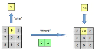
The left is pooling operation, and on the right there is unpooling operation.

but after unpooling operation the unpooled map is a sparse activation map. So we need to deconvolute.
Deconvolution
We do this job via deconvolution layers. They densify the sparse maps with multiple learned filters which is contrary to convolution layers.
The figure below indicates that through deconvolution operation the sparse map are turned into dense map.
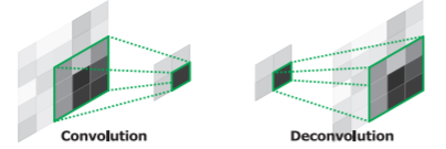
The learned filters in deconvolutional layers correspond to bases to reconstruct shape of an input object.
- The filters in lower layers tend to capture overall shape of an object.
- The filters in higher layers tend to capture the class-specific fine details.
Training
2 tricks are used to train this network on small dataset.
Batch Normalization
- Purpose: reduce the internal-covariate-shift
- Method: normalizing input distributions of every layer to the standard Gaussian distribution.
Two-stage Training
- Attempt:
- the space of semantic segmentation is large compared to the number of training examples.
- the benefit to use a deconvolution network for instance-wise segmentation would be cancelled.
- Method
- First stage:
- crop object instances using ground-truth annotations to…
- center the object at the cropped bounding box.
- limit the variations in object location and size to…
- reduce search space for semantic segmentation
- train the network with much less training examples
- crop object instances using ground-truth annotations to…
- Second stage:
- select candidate proposals sufficiently overlapped with ground-truth segmentations for training to…
- more robust
- yet the location and scale of object may vary across training examples
- select candidate proposals sufficiently overlapped with ground-truth segmentations for training to…
- First stage:
Aggregating Instance-wise Segmentation Maps
Motivation
Some proposals may result in incorrect predictions due to misalignment to object or cluttered background.
Solution
Suppress such noises during aggregation using The pixelwise maximum or average of the score maps.
Ensemble with FCN
Motivation
- Deconvolution network is good at capturing the fine-details of an object.
- FCN is good at extracting the overall shape of an object.
Solution
- Take advantage of the benefit of both algorithms through ensemble.
- We have two sets of class conditional probability maps of input computed independently by the proposed method and FCN.
- Compute the mean of both output maps.
- Apply the CRF to obtain the final semantic segmentation.
PyTorch Implementation Sample of the network “Deconvnet”
import torch
import torchvision.models as models
from torch import nn


vgg16_pretrained = models.vgg16(pretrained=False)
#path_state_dict = os.path.join(BASE_DIR, "data", "vgg16-397923af.pth")
#vgg16_pretrained=get_vgg16(path_state_dict, device, True)


def decoder(input_channel, output_channel, num=3):
    if num == 3:
        decoder_body = nn.Sequential(
            nn.ConvTranspose2d(input_channel, input_channel, 3, padding=1),
            nn.ConvTranspose2d(input_channel, input_channel, 3, padding=1),
            nn.ConvTranspose2d(input_channel, output_channel, 3, padding=1))
    elif num == 2:
        decoder_body = nn.Sequential(
            nn.ConvTranspose2d(input_channel, input_channel, 3, padding=1),
            nn.ConvTranspose2d(input_channel, output_channel, 3, padding=1))

    return decoder_body

# following the designation of deconvnet shown at the beginning of the page
class VGG16_deconv(torch.nn.Module):
    def __init__(self):
        super(VGG16_deconv, self).__init__()

        pool_list = [4, 9, 16, 23, 30]
        for index in pool_list:
            vgg16_pretrained.features[index].return_indices = True

        self.encoder1 = vgg16_pretrained.features[:4]
        self.pool1 = vgg16_pretrained.features[4]

        self.encoder2 = vgg16_pretrained.features[5:9]
        self.pool2 = vgg16_pretrained.features[9]

        self.encoder3 = vgg16_pretrained.features[10:16]
        self.pool3 = vgg16_pretrained.features[16]

        self.encoder4 = vgg16_pretrained.features[17:23]
        self.pool4 = vgg16_pretrained.features[23]

        self.encoder5 = vgg16_pretrained.features[24:30]
        self.pool5 = vgg16_pretrained.features[30]

        self.classifier = nn.Sequential(
            torch.nn.Linear(512 * 11 * 15, 4096),
            torch.nn.ReLU(),
            torch.nn.Linear(4096, 512 * 11 * 15),#512*11*15
            torch.nn.ReLU(),
        )

        self.decoder5 = decoder(512, 512)
        self.unpool5 = nn.MaxUnpool2d(2, 2)

        self.decoder4 = decoder(512, 256)
        self.unpool4 = nn.MaxUnpool2d(2, 2)

        self.decoder3 = decoder(256, 128)
        self.unpool3 = nn.MaxUnpool2d(2, 2)

        self.decoder2 = decoder(128, 64, 2)
        self.unpool2 = nn.MaxUnpool2d(2, 2)

        self.decoder1 = decoder(64, 12, 2)
        self.unpool1 = nn.MaxUnpool2d(2, 2)
# forward propagation
    def forward(self, x):                       # 3, 352, 480
        encoder1 = self.encoder1(x)             # 64, 352, 480
        output_size1 = encoder1.size()          # 64, 352, 480
        pool1, indices1 = self.pool1(encoder1)  # 64, 176, 240

        encoder2 = self.encoder2(pool1)         # 128, 176, 240
        output_size2 = encoder2.size()          # 128, 176, 240
        pool2, indices2 = self.pool2(encoder2)  # 128, 88, 120

        encoder3 = self.encoder3(pool2)         # 256, 88, 120
        output_size3 = encoder3.size()          # 256, 88, 120
        pool3, indices3 = self.pool3(encoder3)  # 256, 44, 60

        encoder4 = self.encoder4(pool3)         # 512, 44, 60
        output_size4 = encoder4.size()          # 512, 44, 60
        pool4, indices4 = self.pool4(encoder4)  # 512, 22, 30

        encoder5 = self.encoder5(pool4)         # 512, 22, 30
        output_size5 = encoder5.size()          # 512, 22, 30
        pool5, indices5 = self.pool5(encoder5)  # 512, 11, 15

        pool5 = pool5.view(pool5.size(0), -1)	#pool5.size(0)=Batchsize,-1
        fc = self.classifier(pool5)
        fc = fc.reshape(1, 512, 11, 15)

        unpool5 = self.unpool5(input=fc, indices=indices5, output_size=output_size5)    # 512, 22, 30
        decoder5 = self.decoder5(unpool5)   # 512, 22, 30

        unpool4 = self.unpool4(input=decoder5, indices=indices4, output_size=output_size4)  # 512, 44, 60
        decoder4 = self.decoder4(unpool4)   # 256, 44, 60

        unpool3 = self.unpool3(input=decoder4, indices=indices3, output_size=output_size3)  # 256, 88, 120
        decoder3 = self.decoder3(unpool3)   # 128, 88, 120

        unpool2 = self.unpool2(input=decoder3, indices=indices2, output_size=output_size2)  # 128, 176, 240
        decoder2 = self.decoder2(unpool2)  # 64, 176, 240

        unpool1 = self.unpool1(input=decoder2, indices=indices1, output_size=output_size1)  # 64, 352, 480
        decoder1 = self.decoder1(unpool1)  # 12, 352, 480

        return decoder1


if __name__ == "__main__":
    import torch as t

    rgb = t.randn(1, 3, 352, 480)

    net = VGG16_deconv()

    out = net(rgb)

    print(out.shape)
Demo
We run a demo of deconvnet as the end of the report.
Before the demo
The source of data in http://cvlab.postech.ac.kr/research/deconvnet/data/ is all removed by the author now. So we can not use his repo https://github.com/HyeonwooNoh/DeconvNet to reproduce his paper now :(
So I find an alternative instead.
Alternative Demo Source
Grad-CAM-pytorch with Deconvnet implementation.
Environment
- Ubuntu 18.04
- Nvidia GeForce GTX1650, 4Gb of GDDR5
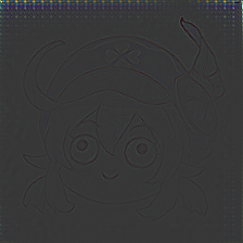
Input
Cute Klee image

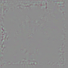
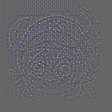
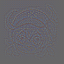
We use the method described in Visualizing and understanding convolutional networks. (ECCV 2014). to take a look at what the inner layer of the network actually look like.
Output
| Predicted class | COMIC BOOK | ENVELOPE | PENCIL BOX |
|---|---|---|---|
| Grad-CAM |  |
 |
 |
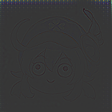
| Vanilla backpropagation | 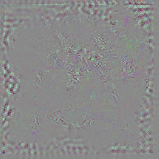 |
 |
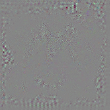 |
| Deconvnet | 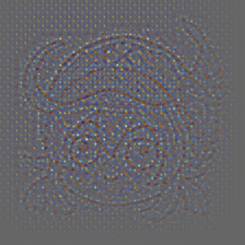 |
 |
 |
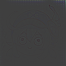
| Guided backpropagation |  |
 |
 |
| Guided Grad-CAM |  |
 |
 |